Overview

In this project we were tasked with implementing the De Casteljau Algorithm for Bezier Curves/Surfaces, and implementing elementary mesh operations (i.e. edge-flip, edge-split, and upsampling) for a Mesh Editor using the halfedge data structure. Succesful implementation of these features is central to processing geometry in computer graphics. Through this project I consolidated my understanding of Bezier curves/surfaces and became fluent with mesh traversal using the halfedge data structure. The images and results shown in this write-up demonstrate the variety of geometric objects and processing schemes that can be acheived using the features implemented herein.

Section I: Bezier Curves and Surfaces

Part 1: Bezier curves with 1D de Casteljau subdivision

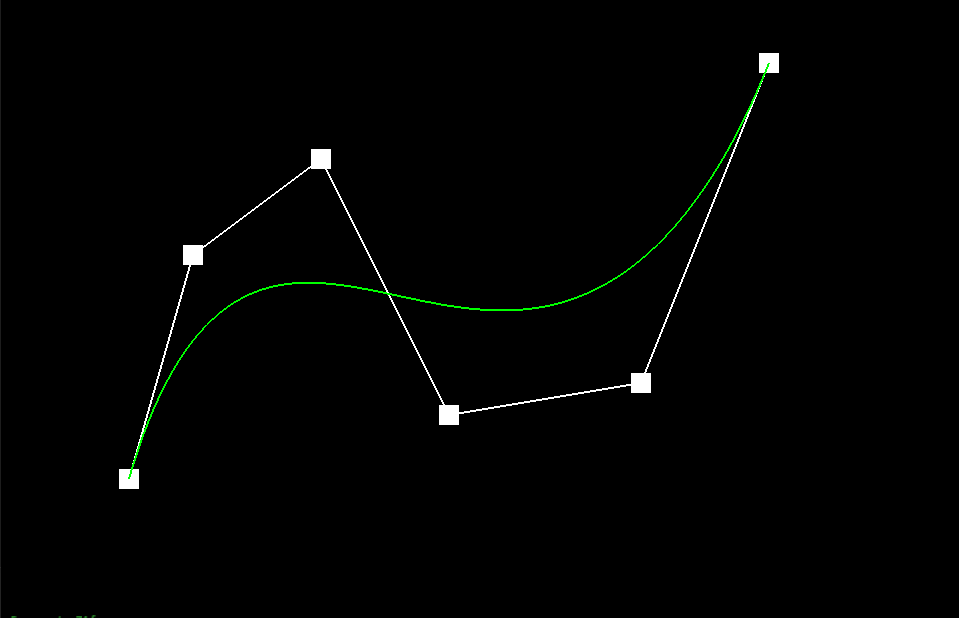
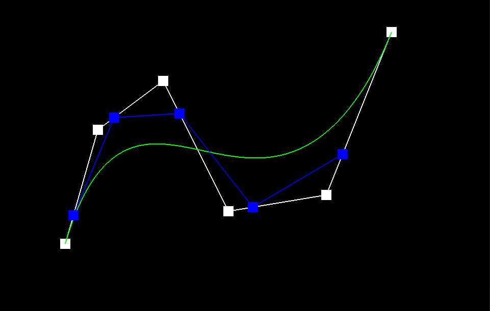
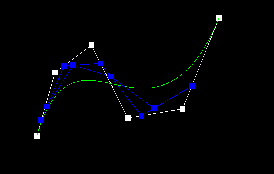
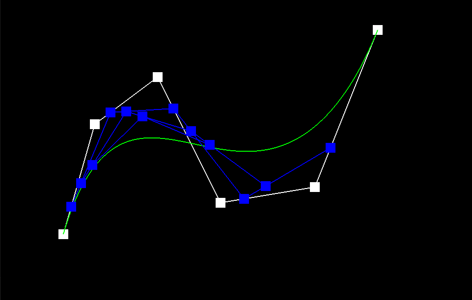
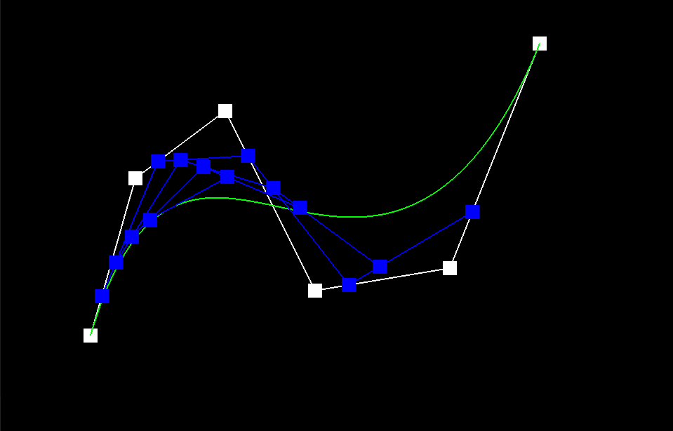
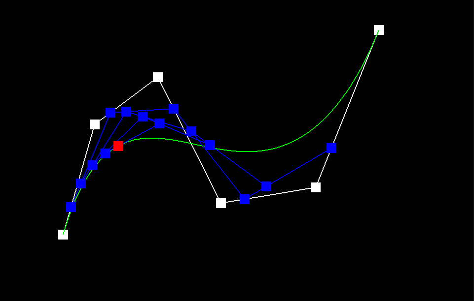
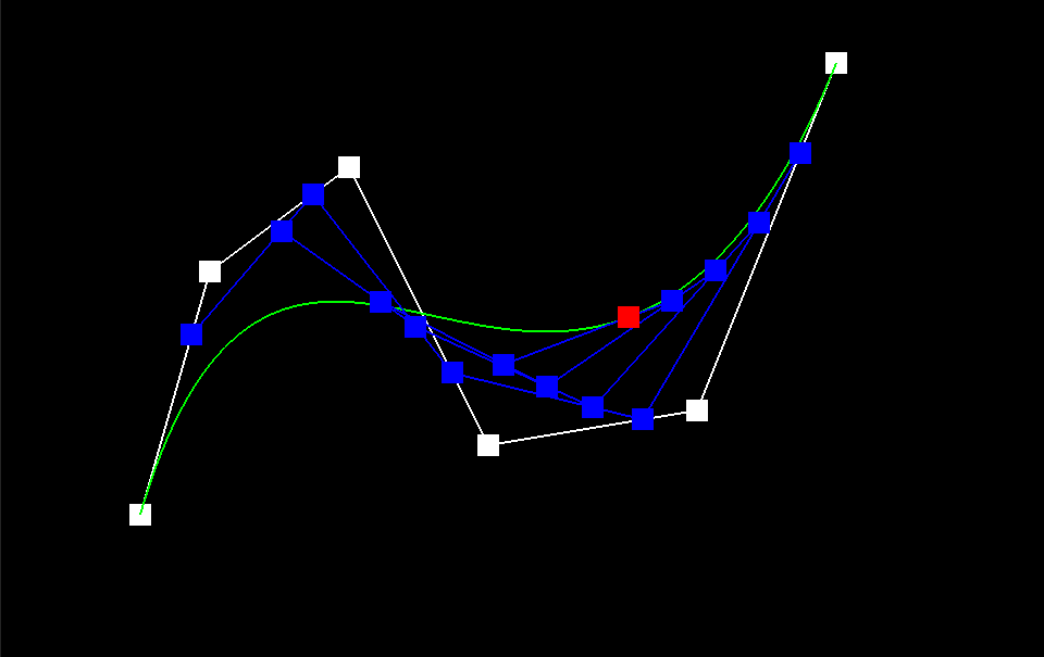
The de Casteljau Algorithm is a technique used to determine the position of a point on a Bezier Curve that is parameterized by the scalar t, which can range from 0 to 1. To achieve this, we start with a list of n control points p_1 ... p_n and recursively interpolate between them, evaluating each line segment at a fractional length t. Mathematically, we define the recursive step as p_i' = (1-t)p_i + tp_i, where the set of primed coordinate points has a length of n-1. To implement this algorithm, we introduce a subroutine called BezierCurve::EvaluateStep() in the BezierCurve class. This subroutine takes in a list of points and a parameter t and performs a single step of the recursion defined earlier, returning a list of linearly-interpolated points. This function is used as a helper for complete descriptions of Bezier Curves and Surfaces. The De Casteljau algorithm converges to a single point on the Bezier curve, as demonstrated by the image sequence below. The green line represents the true Bezier Curve, while the blue line segments in iterations 1-5 show the linear interpolations at each step. The red square in Image 5 indicates the final point on the Bezier curve that the algorithm converges to for a fixed value of t. It is worth noting that this point lies directly on the green reference curve, indicating the algorithm's accuracy.

Part 2: Bezier surfaces with separable 1D de Casteljau subdivision

The 1D De Casteljau Algorithm can be extended to 2D Bezier surfaces by defining the surface using an assortment of 1D Bezier curves. In 3D space, given a collection of m Bezier curves each defined with n control points and parametrized by a scalar u, we can define a Bezier surface as the locus of points reached by a 'sliding' Bezier curve g_u(v) defined through the control points p_1 = f_1(u), p_2 = f_2(u), ...,p_m = f_m(u) for a fixed u. By letting u vary, we have a function of 2 coordinates, g(uv).

To evaluate a point g(u,v) on such surfaces using the De Casteljau Algorithm, we define a function that takes in an mxn 2D vector of control points and the parametric coordinates (u,v). The 1D De Casteljau algorithm is first executed along the rows of the 2D vector, which results in a set of m Bezier curves evaluated at u. Then using these resulting m points, the 'sliding' Bezier curve is evaluated at v with the De Casteljau Algorithm. The resulting point is the desired point on the Bezier surface. By creating a patchwork of Bezier surfaces, complex geometries with hard edges, beveled surfaces, and discontinuities can be achieved, as demonstrated in the image below.

Section II: Sampling

Part 3: Average normals for half-edge meshes

The implementation of vertex normals involved utilizing the halfedge data structure and properties of vector cross-products. To begin, we accessed the vertex in the mesh and traversed the faces surrounding it. We retrieved the normal vectors associated with each face and calculated their weights based on the area of the corresponding face. To access the surrounding faces, we retrieved the halfedge associated with the target vertex and iterated through the outgoing halfedges. Using the halfedge mesh representation, we accessed the normal vectors associated with each face. Next, determining the area of each face to calculate the appropriate weighting factor for the normal vectors, we used the geometric relationship between the magnitude of the cross-product of two vectors and twice the area of the triangle defined by the two vectors. Since the cross-product operation itself produces a vector normal to the plane contained by the two argument vectors, it was unnecessary to retrieve the normal from the face element. Finally, we computed the vertex normal by performing a weighted sum of the normal vectors of each face, where the weights corresponded to the fractional area of the face. The shading benefits of using vertex normals are evident when comparing the before and after images. Our implementation produced smoother and more realistic shading, as opposed to the flat shading produced by the default normal calculation. By calculating the normal at each vertex, the smoothness of the surface is increased, as the lighting of each vertex is dependent on the surrounding faces. This produces more realistic and natural-looking lighting, as opposed to the artificial-looking lighting produced by flat shading.

Part 4: Half-edge flip

To implement the edge-flip operation on the mesh, precise pointer manipulation was necessary. We initially drew the old and new triangle after flipping by hand and recorded the reassignments required for each element involved in the operation. This drawing served as a visual guide for the pointer manipulations that needed to be performed. To ensure that the edge being flipped was not a boundary edge, I added a check. Using traversal functions for the halfedge mesh, we then created temporary variables for all relevant mesh elements. With these variables, we executed the previously recorded reassignments accurately. Thankfully, we encountered no major bugs during this meticulous process, all of the bugs were related to pointers, which the drawing helped prevented against.

Part 5: Half-edge split

To execute the edge split operation, we followed a comparable procedure to that outlined for the edge-flip operation. Nevertheless, this process involves adding 1 new vertex, 3 new edge components, and 6 new halfedges to the mesh. Upon computing the pointer reassignments for each mesh component, we positioned the new vertex at the midpoint of the target edge and marked all newly generated edges (except new edges created from the old edge) and vertices as new by setting their isNew field to true to help with then Loop subdivision in Part 6.

Part 6: Loop subdivision for mesh upsampling

As instructed in the project specifications, we started the mesh subdivision process by preprocessing the vertex locations of both the old and new vertices in the target mesh. For the old vertices, we saved the new locations in the "newPosition" field of the vertices themselves. We put the new locations of the new vertices inside the Edge that will be splitted. This way, they could be accessed after edge-splits and would be connected to the new vertices. Then, we went through all the old edges of the mesh and split them using the edge-split operation. It took me a while to deal with infinite loops caused by adding new edges to the mesh, but We eventually set the proper conditions for splitting an edge (i.e. making sure none of the vertices at both ends of the edge were new). After that, we spent some time figuring out the conditions for flipping an edge, We updated my splitEdge function to mark the new edges that bisected the original edge as "isNew" as mentioned above and flipped only the new edges that connecting between an old vertex and a new vertex (as what it should be conceptually). Finally, we repositioned each vertex using the preprocessed locations identified at the beginning.

When applying loop subdivision to a mesh, the process involves repositioning vertices to make the mesh more uniformly sampled. As a result, sharp edges become rounded. We can view the sharp edges as high frequency 3D content in the mesh. By enforcing mesh uniformity (i.e. making the spacing between vertices roughly consistent), we effectively impose a Nyquist sampling frequency. Therefore, loop subdivision bevels sharp edges and tends to produce the most quadric error after the first iteration. The images of the cube below illustrate this effect. Additionally, by comparing the first and second sets of the image sequence, we can observe the differences. This distinction can be attributed to the starting topology of the cube for each case. In the first set, where the cube geometry converges to an asymmetric convex body, there are only two triangles per face of the cube and two rotationally symmetric configurations over each cartesian axis. In contrast, in the second set, where the cube geometry converges to a more symmetric convex body, there are sixteen triangles per cube face and four rotationally symmetric configurations over each cartesian axis. Therefore, since the second set cube topology contains more samples than the first set cube topology, upsampling results in an object that is more cube-like.