In this project, we developed a radiometrically accurate ray-tracing pipeline for rendering virtual scenes. The pipeline is composed of five parts, each of which contain specific optimizations to improve render efficiency and quality. Overall, these parts, and their effects on the render, are presented in the chronology in which they are executed within the pipeline. The images shown herein attempt to visually demonstrate the role of each step of the render. The differences in render quality and efficiency achieved through the progression of algorithms explored in this project are salient.

Part 1: Ray Generation and Scene Intersection

Walk through the ray generation and primitive intersection parts of the rendering pipeline.

In order to generate a ray, we need two pieces of information: the origin coordinate (which is the camera's position in world space) and a direction vector that has been normalized. When using ray casting to sample every pixel, we need to perform three mappings to determine the appropriate ray direction for each pixel. The first mapping transforms the pixel coordinates into a normalized coordinate frame by scaling the axes. The second mapping takes the normalized coordinate frame and transforms it into the image frame, which defines the field of view captured in the scene. This transformation is accomplished by scaling and translating perpendicular to the camera's Z axis. The goal of these first two transformations is to align the pixel plane with the image plane, allowing us to draw a ray from the camera origin through the field of view for any given pixel. To sample multiple times for a single pixel, we can perturb the ray direction within the bounds of the pixel area. Once the ray direction for the pixel is determined, we apply the camera-to-world transformation to the direction vector so that the ray travels properly through the scene. The origin of the ray is also translated to match the camera's origin.

Explain the triangle intersection algorithm you implemented in your own words.

To find where rays intersect with triangles, the Moller-Trumbore Algorithm was implemented, which combines Barycentric coordinates and an implicit plane definition to determine if the intersection point is inside the triangle. To confirm an intersection with a triangle primitive, the Barycentric Coordinates were checked to ensure they were within the range [0,1], and the intersection t-value was checked to be within the maximum and minimum bounds of the scene. Sphere intersection checks were more complex. First, the intersection t-values were found by solving a quadratic equation using the quadratic root formula. The discriminant was checked to ensure it was non-negative, indicating the solution had at least one real root. Then, it was checked if either of the roots of the quadratic equation fell within the max and minimum bounds. Finally, the minimum root was selected if both roots satisfied the previous conditions.

Show images with normal shading for a few small .dae files

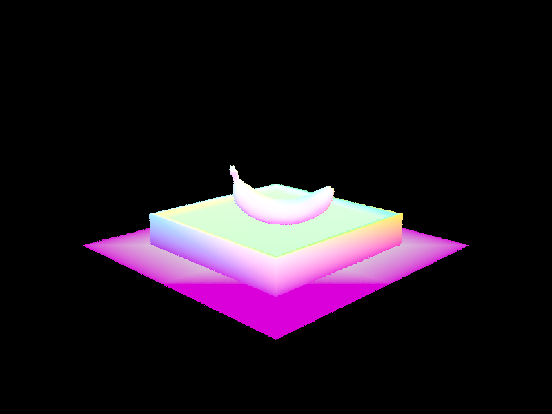
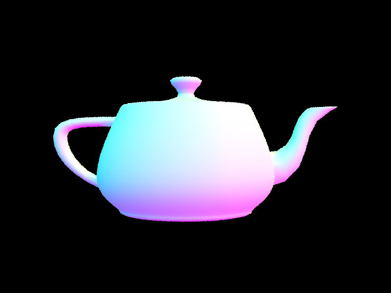
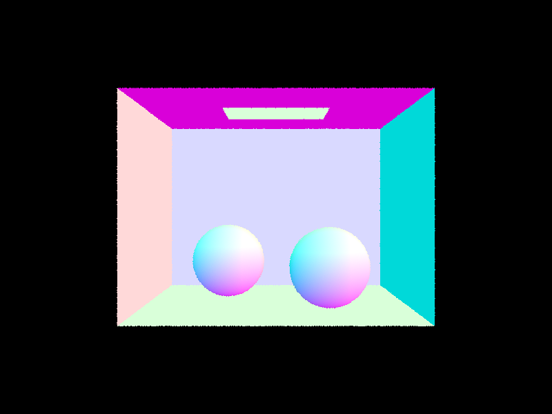
Part 2: Bounding Volume Hierarchy

Walk through your BVH construction algorithm. Explain the heuristic you chose for picking the splitting point.

The efficiency of ray tracing was greatly enhanced by utilizing a heuristic for determining the BVH split point. To begin with, we calculated the average 3D position of the centroids of all the primitives enclosed in the bounding box of a given BVH node. This enabled us to identify three possible split points along the x, y, and z axes. We created the helpers function that allows us to sort the primitives based on their x, y, x axes. From that, we split the bounding box along the axis that has the greatest distance (e.g. max - min) into two child bounding boxes with equal (give or take) numbers of primitives. The images below illustrate the 3-axis heuristic bounding boxes, making them more tightly encompass the primitives. As a result, the likelihood of a ray striking the bounding box of a BVH but not hitting a primitive was reduced, and the density of primitives per bounding box was significantly enhanced.

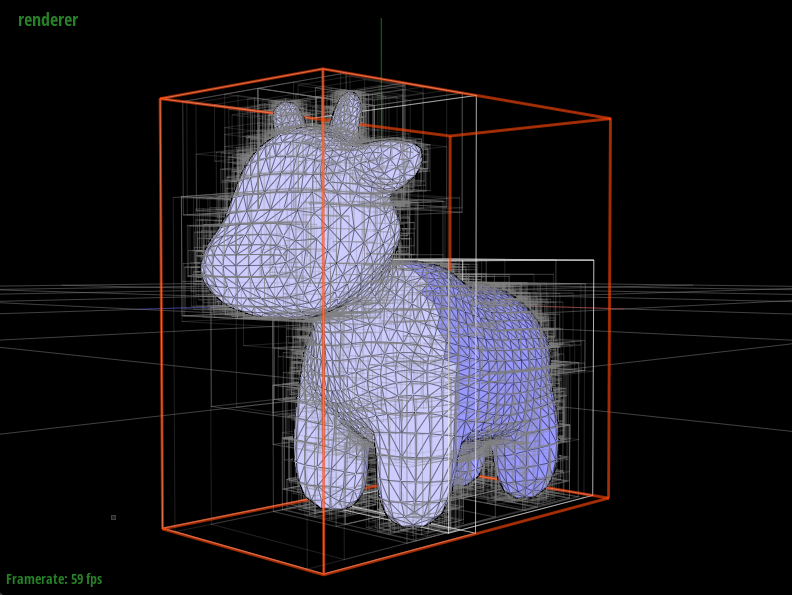
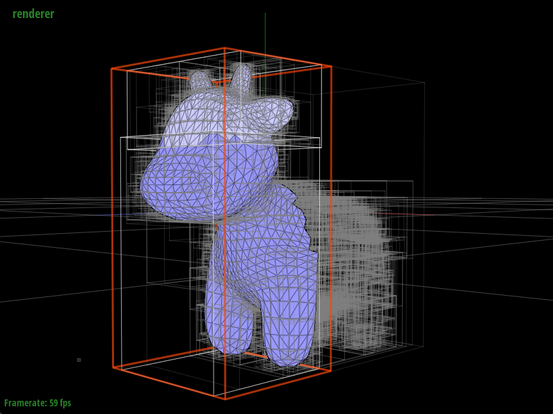
Compare rendering times on a few scenes with moderately complex geometries with and without BVH acceleration. Present your results in a one-paragraph analysis.

The computational efficiency of rendering is significantly improved with the implementation of a BVH. For example, the rendering of the cow below was completed in 38.1913 seconds without the BVH, compared to just 0.1249 seconds with the BVH. In addition, the average number of ray intersection tests was approximately 942 without the BVH, compared to only 3.4 intersection tests with the BVH. The BVH approach is attractive due to its lower computational complexity. Without the BVH, the average number of intersection tests per ray is O(n), while with a BVH, the computational complexity is O(logn), where n is the number of primitives in the scene. This enables the scaling of mesh complexity and resolution without significantly affecting the rendering time.

Show images with normal shading for a few large .dae files that you can only render with BVH acceleration.

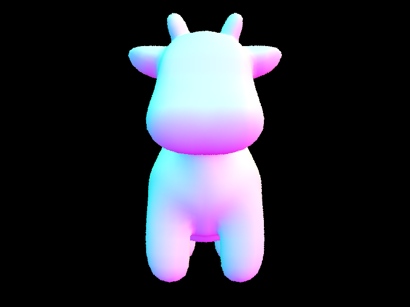
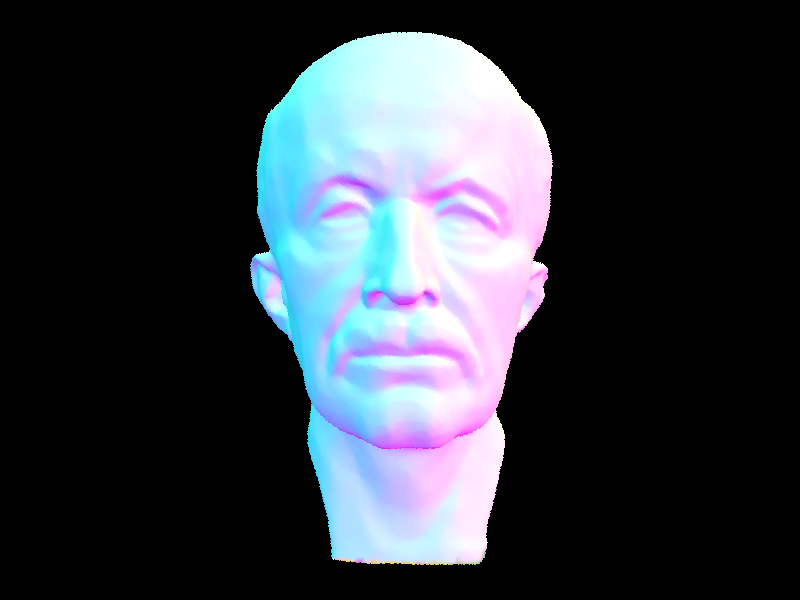
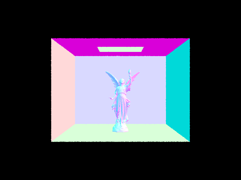
Part 3: Direct Illumination

Walk through both implementations of the direct lighting function.

In this project, direct lighting refers to the calculation of illumination produced by light rays that bounce one time or less on scene objects before arriving at the image plane. We explored two approaches to direct lighting: Uniform Hemisphere sampling and Importance sampling. These methods differ in how they sample the incident light ray directions for approximating the reflection equation using Monte-Carlo integration. In both approaches, we consider the inverse light path of a ray originating at the camera and entering the scene. When the ray intersects an object in the scene, the radiance that the camera observes leaving this point of intersection depends on the Bidirectional Radiance Distribution Function (BRDF) of the object's surface and the irradiance arriving at that point. To estimate the Monte-Carlo integral, we sample several ray directions in the object coordinate space and propagate new rays in those directions until they reach a light source. If the rays are obstructed, they are considered shadow rays and do not contribute to the integral. With Uniform Hemisphere sampling, the direction of the sampling rays is not guaranteed to point towards the light source. Therefore, many of the explored rays may not contribute anything to the reflection equation integral. In contrast, Importance sampling generates sampling rays that are guaranteed to point towards the light source. These rays are only excluded if there is an obstruction, thus better characterizing the overall irradiance with the same number of samples.

In this project, we have only implemented a BRDF for diffuse Lambertian reflection. Hence, the BRDF is for diffuse surfaces is independent of the incident and outgoing ray directions. Therefore, the only terms in the reflection integral that do depend on the incident ray direction are L, the incident radiance, and the Lambertian cosine factor. These quantities were thus computed once the ray direction in object space was sampled.

Compare the results between uniform hemisphere sampling and lighting sampling in a one-paragraph analysis.

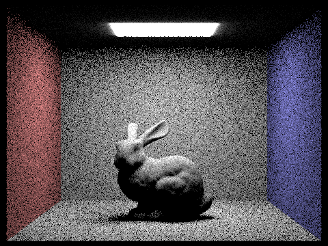
The direct illumination images shown below compare renders involving the Uniform Hemisphere sampling and Importance sampling techniques described previously for different numbers of pixel samples and light samples. Noise in the renders is substantially reduced when using importance sampling. This demonstrates the effectiveness of the importance sampling technique in producing drastically higher render quality for the same number of samples.

Show some images rendered with both implementations of the direct lighting function.

Focus on one particular scene with at least one area light and compare the noise levels in soft shadows when rendering with 1, 4, 16, and 64 light rays (the -l flag) and with 1 sample per pixel (the -s flag) using light sampling, not uniform hemisphere sampling.

Importance Sampling Renders - Bunny Scene

Part 4: Global Illumination

Walk through your implementation of the indirect lighting function.

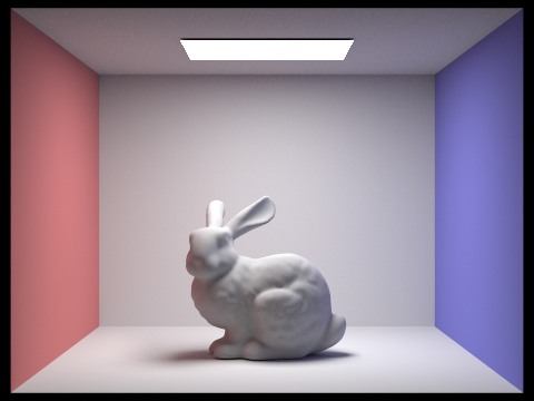
Indirect Illumination refers to the inclusion of light reflections between non-emitting objects in a scene. In order to achieve this, ray-tracing for indirect illumination uses a recursive method to explore all possible light paths from the source to the camera. The indirect lighting function works as follows:

• When a non-emitting object in the scene is intersected, the direct-lighting contribution at that point is collected.
• A weighted coin is then flipped to determine whether to continue tracing rays. This unbiased probabilistic termination criterion, known as the Russian Roulette approach, prevents infinite recursion.
• IIf ray-tracing is to be continued, directions are randomly sampled from the intersection point, and rays are propagated in those directions until another non-emitting object is reached.
• The process is then repeated recursively on the new intersection point.

Indirect illumination improves the realism of rendered images by accounting for multiple light bounces. This is particularly evident in the color bleeding from the red and blue walls onto the subject, as well as the softer shadowing, when comparing the direct illumination with the global illumination renderings of the bunny shown below. The second row of images isolates the contributions from single-bounce (direct illumination), two-bounce, and three-bounce light paths to emphasize their relative importance. The final image is the sum of these images and the zero-bounce contribution, representing ray paths that travel directly between the area light source and the camera.

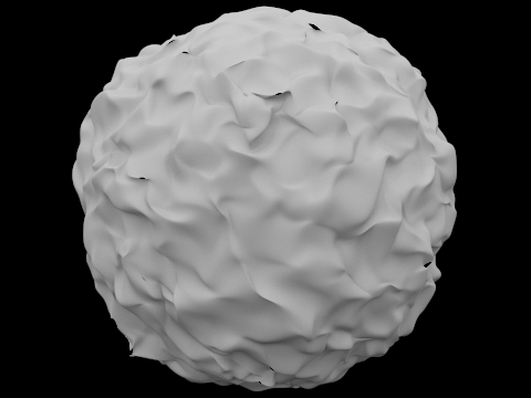
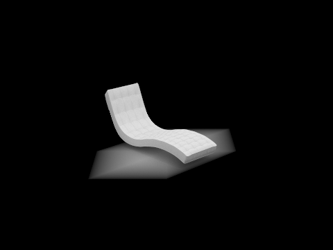
Show some images rendered with global (direct and indirect) illumination. Use 1024 samples per pixel.

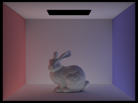
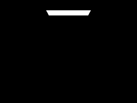
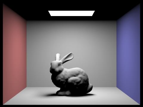
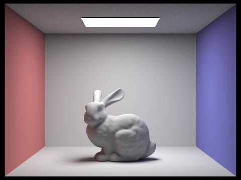
Pick one scene and compare rendered views first with only direct illumination, then only indirect illumination. Use 1024 samples per pixel.

For CBbunny.dae, compare rendered views with max_ray_depth set to 0, 1, 2, 3, and 100 (the -m flag). Use 1024 samples per pixel.

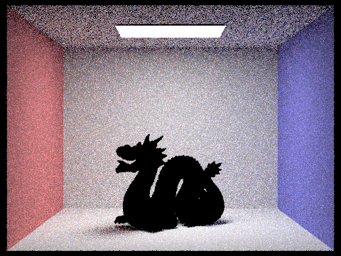
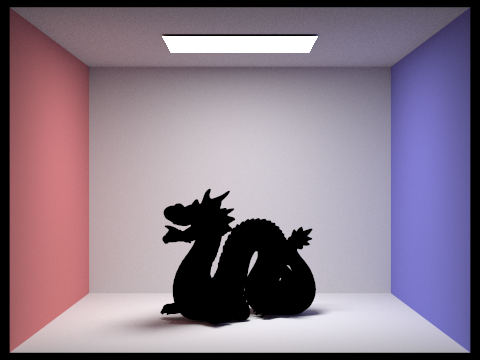
Pick one scene and compare rendered views with various sample-per-pixel rates, including at least 1, 2, 4, 8, 16, 64, and 1024. Use 4 light rays.

Part 5: Adaptive Sampling

Explain adaptive sampling. Walk through your implementation of the adaptive sampling.

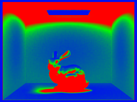
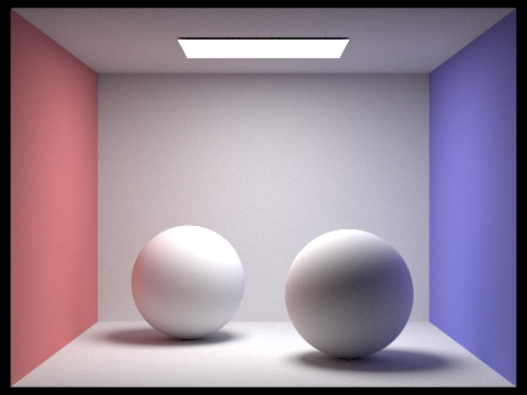
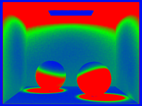
The technique of adaptive sampling efficiently reduces the number of rays processed per pixel by monitoring the convergence behavior of each pixel's illuminance. If a pixel has stabilized at a certain value, it does not require further sampling to achieve high-fidelity rendering of the scene. To implement adaptive sampling, we made modifications to the raytrace_pixel() function such that it terminates its sample-averaging loop before reaching the maximum number of samples if the convergence conditions for illuminance are met. These conditions are based on the average illuminance, variance in the samples, and z-scores, assuming a Gaussian probability distribution of illuminance within the pixel footprint. Adaptive sampling optimizes the amount of pixel super-sampling, improving computational efficiency while marrying the variation of information within a single pixel's scene footprint with the degree of super-sampling required for that pixel.

Pick two scenes and render them with at least 2048 samples per pixel. Show a good sampling rate image with clearly visible differences in sampling rate over various regions and pixels. Include both your sample rate image, which shows your how your adaptive sampling changes depending on which part of the image you are rendering, and your noise-free rendered result. Use 1 sample per light and at least 5 for max ray depth.